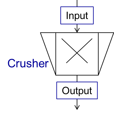
Crusher

A crusher comminutes the input material stream and reduces the average particle size. The schema is illustrated below.

This unit can be described using 3 models in Dyssol:

Bond’s model

Cone model

Const model

Bond’s model

This model is used to perform milling of the input stream. The crushing is performed according to the model proposed by Bond. The simplification is made, and the particle size distribution of the output stream is described by the normal function.

$x_{80,out} = \dfrac{1}{ \left( \dfrac{P}{10\,w_i\,\dot{m}} + \dfrac{1}{\sqrt{x_{80,in}}} \right)^2}$

$\mu = x_{80,out} - 0.83\sigma$

$q_3(x) = \frac{1}{\sigma\sqrt{2\pi}}\,e^{-\dfrac{(x-\mu)^2}{2\sigma^2}}$

Note

Notations applied in this model:

$x_{80,out}$ – characteristic particle size of the output stream

$x_{80,in}$ – characteristic particle size of the input stream

$w_i$ – Bond Work Index, dependent on the material

$P$ – power input

$\dot{m}$ – mass flow of solids in the input stream

$q_3(x)$ – output mass related density distribution

$\sigma$ – standard deviation of the output normal distribution

$\mu$ – mean value of the output normal distribution

Note

Solid phase and particle size distribution are required for the simulation.

Note

Input parameters needed for the simulation:

Name	Symbol	Description	Units	Boundaries
P	$P$	Power input	[kW]	P > 0
Wi	$w_i$	Bond work index	[kWh/t]	1 ≤ Wi ≤ 100
Standard deviation	$\sigma$	Standard deviation of the output distribution	[m]	Standard deviation > 0

See also

a demostration file at Example Flowsheets/Units/Crusher Bond.dlfw.

See also

F.C. Bond, Crushing and grinding calculation – Part I, British Chemical Engineering 6 (6) (1961) 378-385.
F.C. Bond, Crushing and grinding calculation – Part II, British Chemical Engineering 6 (8), (1961) 543-548.
Denver Sala Basic: Selection Guide for Process Equipment, 1993.

Average Bond Work Indices for various materials

Material	Work Bond Index [kWh/t]	Material	Work Bond Index [kWh/t]
Andesite	20.08	Iron ore, oolitic	12.46
Barite	5.2	Iron ore, taconite	16.07
Basalt	18.18	Lead ore	13.09
Bauxite	9.66	Lead-zinc ore	12.02
Cement clinker	14.8	Limestone	14
Clay	6.93	Manganese ore	13.42
Coal	14.3	Magnesite	12.24
Coke	16.84	Molybdenum	14.08
Copper ore	13.99	Nickel ore	15.02
Diorite	22.99	Oil shale	17.43
Dolomite	12.4	Phosphate rock	10.91
Emery	62.45	Potash ore	8.86
Feldspar	11.88	Pyrite ore	9.83
Ferro-chrome	8.4	Pyrrhotite ore	10.53
Ferro-manganese	9.13	Quartzite	10.54
Ferro-silicon	11	Quartz	14.93
Flint	28.78	Rutile ore	13.95
Fluorspar	9.8	Shale	17.46
Gabbro	20.3	Silica sand	15.51
Glass	13.54	Silicon carbide	27.46
Gneiss	22.14	Slag	11.26
Gold ore	16.42	Slate	15.73
Granite	16.64	Sodium silicate	14.74
Graphite	47.92	Spodumene ore	11.41
Gravel	17.67	Syenite	14.44
Gypsum rock	7.4	Tin ore	11.99
Iron ore ,hematite	14.12	Titanium ore	13.56
Iron ore, hematite-specular	15.22	Trap rock	21.25
Iron ore, magnetite	10.97	Zinc ore	12.72

Cone model

The model is described below as

$w_{out,i} = \sum\limits^{i}_{k=0} w_{in,k} \cdot S_k \cdot B_{ki} + (1-S_i)\,w_{in,i}$

Note

Notations:

$w_{out,i}$ – mass fraction of particles with size $i$ in output distribution

$w_{in,i}$ – mass fraction of particles with size $i$ in inlet distribution

$S_k$ – mass fraction of particles with size $k$ , which will be crushed

$B_{ki}$ – mass fraction of particles with size $i$ , which get size after breakage less or equal to $k$

$S_k$ is described by the King selection function.

$S_k = \begin{cases} 0 & x_k \leqslant x_{min} \\ 1 - \dfrac{x_{max} - x_i}{x_{max} - x_{min}} & x_{min} < x_k < x_{max} \\ 1 & x_k \geqslant x_{max} \end{cases}$

$x_{min} = CSS \cdot \alpha_1 x_{max} = CSS \cdot \alpha_2$

Note

Notations:

$x_k$ – mean particle diameter in size-class $k$

$CSS$ – close size setting of a cone crusher

$\alpha_1, \alpha_2, n$ – parameters of the King selection function

$B_{ki}$ is calculated by the Vogel breakage function.

$B_{ki} = \begin{cases} 0.5\, \left( \dfrac{x_i}{x_k} \right)^q \cdot \left( 1 + \tanh \left( \dfrac{x_k - x'}{x'} \right) \right) & i \geqslant k \\ 0 & i < k \end{cases}$

Note

Notations:

$x'$ – minimum fragment size which can be achieved by crushing

$q$ – parameter of the Vogel breakage function

Note

Solid phase and particle size distribution are required for the simulation.

Note

Input parameters needed for the simulation:

Name	Symbol	Description	Units	Boundaries
CSS	$CSS$	Close size setting of a cone crusher. Parameter of the King selection function	[m]	CSS > 0
alpha1	$\alpha_1$	Parameter of the King selection function	[–]	0.5 ≤ alpha1 ≤ 0.95
alpha2	$\alpha_2$	Parameter of the King selection function	[–]	1.7 ≤ alpha2 ≤ 3.5
n	$n$	Parameter of the King selection function	[–]	1 ≤ n ≤ 3
d’	$x'$	Minimum fragment size achieved by crushing. Parameter of the Vogel breakage function	[m]	d’ > 0
q	$q$	Parameter of the Vogel breakage function	[–]

See also

a demostration file at Example Flowsheets/Units/Crusher Cone.dlfw.

See also

King, R. P., Modeling and simulation of mineral processing systems, Butterworth & Heinemann, Oxford, 2001.
Vogel, L., Peukert, W., Modelling of Grinding in an Air Classifier Mill Based on A Fundamental Material Function, KONA, 21, 2003, 109-120.

Const output model

This model sets a normal distribution with the specified constant parameters to the output stream. Outlet distribution does not depend on the inlet distribution.

$q_3(x) = \frac{1}{\sigma\sqrt{2\pi}}\,e^{-\dfrac{(x-\mu)^2}{2\sigma^2}}$

Note

Notations:

$q_3(x)$ – output mass related density distribution

$\sigma$ – standard deviation of the output normal distribution

$\mu$ – mean value of the output normal distribution

Note

Solid phase and particle size distribution are required for the simulation.

Note

Input parameters needed for the simulation:

Name	Symbol	Description	Units	Boundaries
Mean	$\mu$	Mean of the normal output distribution	[m]	Mean > 0
Standard deviation	$\sigma$	Standard deviation of the normal output distribution	[m]	Standard deviation > 0

See also

a demostration file at Example Flowsheets/Units/Crusher Const.dlfw.