Time delay

Constant delay of input signal

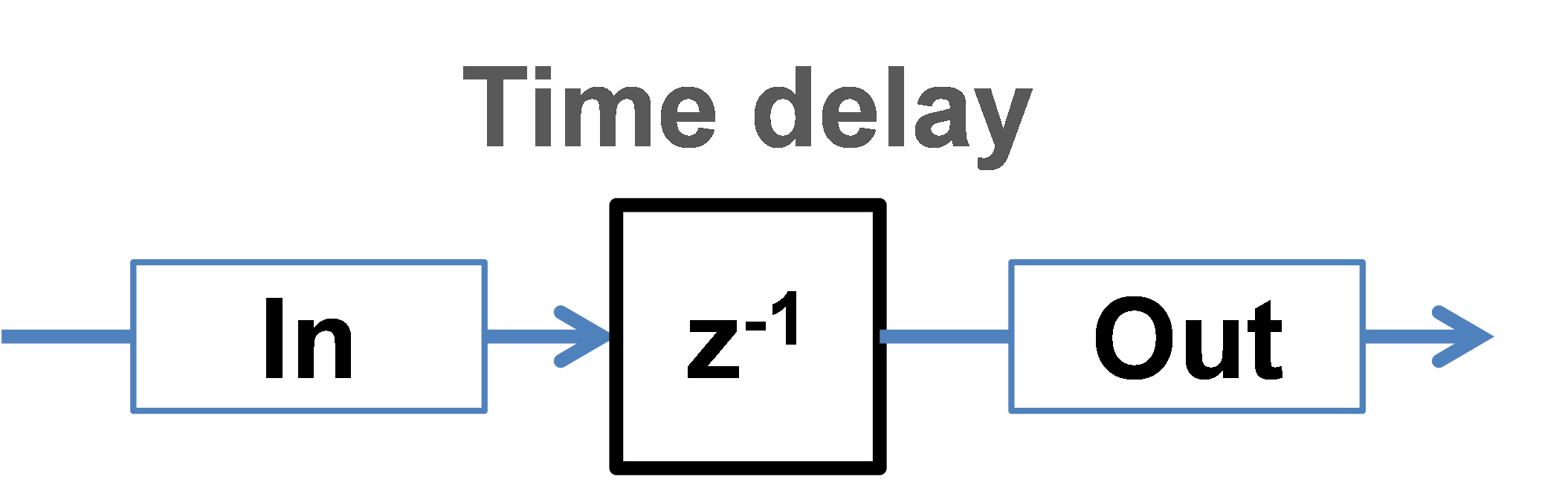
Simple shift

Copies all time points \(t\) from the input stream \(In\) to the output stream \(Out\) at the timepoint \(t + \Delta t\), delaying the signal by a constant value \(\Delta t\).

Norm-based

\[\frac{dm}{dt} = \dot{m}_{in}(t-\Delta t) - m\]

To correctly take into account the dynamics of the process, norms of each overall parameter (mass flow, temperature, pressure) are maintained as:

\[\frac{d||X||}{dt} = (X(t) - X(t-1))^2 - ||X||\]

For phase fractions:

\[\frac{d||P||}{dt} = \sqrt{\sum_{i}^{N_{P}}{(w_{i}(t) - w_{i}(t-1))^2}} - ||P||\]

For compound fractions in each phase:

\[\frac{d||C_{i}||}{dt} = \sqrt{\sum_{j}^{N_{C_{i}}}{(w_{i,j}(t) - w_{i, j}(t-1))^2}} - ||C||\]

For each distributed parameter:

\[\frac{d||D_{i}||}{dt} = \sqrt{\sum_{j}^{N_{D_{i}}}{(w_{i,j}(t) - w_{i,j}(t-1))^2}} - ||D||\]

Note

Notations:

\({m}\) – current mass

\(\dot{m}_{in}\) – input mass flow

\(\Delta t\) – time delay

\(X(t)\) – value of an overall parameter at time point \(t\)

\(w(t)\) – mass fraction at time point \(t\)

\(N_{P}\) – number of defined phases

\(N_{C_{i}}\) – number of defined compounds in phase \(i\)

\(N_{D_{i}}\) – number of classes in distribution \(i\)

Note

Model parameters:

Name	Symbol	Description	Units	Boundaries
Time delay		Model to use		Norm based, Simple shift
Time delay	\(\Delta t\)	Time delay	[s]	>=0
Relative tolerance		Relative tolerance for DAE solver	[-]	>0 (0 for flowsheet-wide value)
Absolute tolerance		Absolute tolerance for DAE solver	[-]	>0 (0 for flowsheet-wide value)