Screen

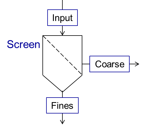
Screen unit is designed for classification of input material into two fractions according to particle size distribution (PSD), as shown below.

There are several models available to describe the screen grade efficiency:

Plitt’s model

Molerus & Hoffmann model

Probability model

Teipel / Hennig model

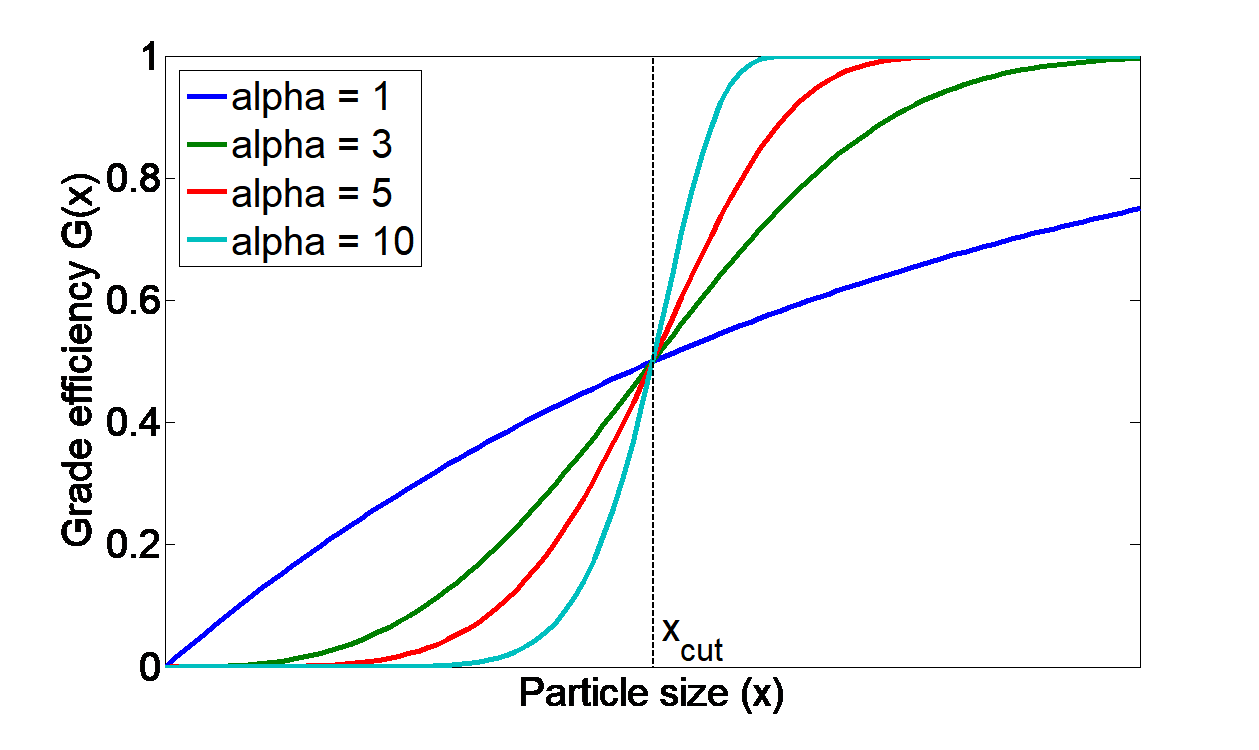
In the following figure, several grade efficiency curves for different parameters of separations sharpness are shown.

Note

This figure only applies to the Plitt’s model and Molerus & Hoffmann model.

The output mass flows are calculated as follows:

$\dot{m}_{out,c} = \dot{m}_{in}\sum\limits_{i}G(x_i)w_{in,i}$

$\dot{m}_{out,f} = \dot{m}_{in}\left(1-\sum\limits_{i}G(x_i)w_{in,i}\right)$

Note

Notations:

Symbol	Units	Description
$\dot{m}_{out,c}$	[kg/s]	Mass flow at the coarse output
$\dot{m}_{out,f}$	[kg/s]	Mass flow at the fine output
$\dot{m}_{in}$	[kg/s]	Feed mass flow
$G(x_i)$	[kg/kg]	Grade efficiency: mass fraction of material of size class $i$ in the feed that leaves the screen in the coarse stream
$w_{in,i}$	[kg/kg]	Mass fraction of material of size class $i$ in the feed

Plitt’s model

This model is described using the following equation:

$G(x_i) = 1 - exp\left(-0.693\,\left(\frac{x_i}{x_{cut}}\right)^\alpha\right)$

Note

Notations applied in the models:

$G(x_i)$ – grade efficiency

$x_{cut}$ – cut size of the classification model

$\alpha$ – sharpness of separation

$x_i$ – size of a particle

Note

Input parameters needed for the simulation:

Name	Symbol	Description	Units	Boundaries
Xcut	$x_{cut}$	Cut size of the classification model	[m]	Xcut > 0
Alpha	$\alpha$	Sharpness of separation	[–]	0 ≤ Alpha ≤ 100

See also

a demostration file at Example Flowsheets/Units/Screen Plitt.dlfw.

See also

Plitt, L.R.: The analysis of solid–solid separations in classifiers. CIM Bulletin 64 (708), p. 42–47, 1971.

Molerus & Hoffmann model

This model is described using the following equation:

$G(x_i) = \dfrac{1}{1 + \left( \dfrac{x_{cut}}{x_i} \right)^2 \cdot exp\left( \alpha \,\left( 1 - \left(\dfrac{x_i}{x_{cut}}\right)^2 \right)\right)}$

Note

Notations applied in the models:

$G(x_i)$ – grade efficiency

$x_{cut}$ – cut size of the classification model

$\alpha$ – sharpness of separation

$x_i$ – size of a particle

Note

Input parameters needed for the simulation:

Name	Symbol	Description	Units	Boundaries
Xcut	$x_{cut}$	Cut size of the classification model	[m]	Xcut > 0
Alpha	$\alpha$	Sharpness of separation	[–]	0 < Alpha ≤ 100

See also

a demostration file at Example Flowsheets/Units/Screen Molerus-Hoffmann.dlfw.

See also

Molerus, O.; Hoffmann, H.: Darstellung von Windsichtertrennkurven durch ein stochastisches Modell, Chemie Ingenieur Technik, 41 (5+6), 1969, pp. 340-344.

Probability model

This model is described using the following equation:

$G(x_i) = \dfrac{ \sum\limits^{x_i}_{0} e^{-\dfrac{(x_i - \mu)^2}{2\sigma^2}} }{ \sum\limits^{N}_{0} e^{-\dfrac{(x_i - \mu)^2}{2\sigma^2}} }$

Note

Notations applied in this model:

$G(x_i)$ – grade efficiency

$x_i$ – size of a particle

$\sigma$ – standard deviation of the normal output distribution

$\mu$ – mean of the normal output distribution

$N$ – number of classes of particle size distribution

Note

Input parameters needed for the simulation:

Name	Symbol	Description	Units	Boundaries
Mean	$\mu$	Mean of the normal output distribution	[m]	Mean > 0
Standard deviation	$\sigma$	Standard deviation of the normal output distribution	[m]	Standard deviation > 0

See also

a demostration file at Example Flowsheets/Units/Screen Probability.dlfw.

See also

Radichkov, R.; Müller, T.; Kienle, A.; Heinrich, S.; Peglow, M.; Mörl, L.: A numerical bifurcation analysis of continuous fluidized bed spray granulation with external product classification, Chemical Engineering and Processing 45, 2006, pp. 826–837.

Teipel / Hennig model

This model is described using the following equation:

$G(x_i) = \left( 1- \left( 1 + 3 \cdot \left( \dfrac{x_i}{x_{cut}} \right)^{\left(\dfrac{x_i}{x_{cut}} + \alpha \right)\cdot \beta} \right)^{-1/2}\right) \cdot (1 - a) + a$

Note

Notations applied in the models:

$G(x_i)$ – grade efficiency

$x_{cut}$ – cut size of the classification model

$\alpha$ – sharpness of separation

$\beta$ - sharpness of separation

$a$ - separation offset

$x_i$ – size of a particle

Note

Input parameters needed for the simulation:

Name	Symbol	Description	Units	Boundaries
Xcut	$x_{cut}$	Cut size of the classification model	[m]	Xcut > 0
Alpha	$\alpha$	Sharpness of separation 1	[–]	0 < Alpha ≤ 100
Beta	$\beta$	Sharpness of separation 2	[–]	0 < Beta ≤ 100
Offset	$a$	Separation offset	[–]	0 ≤ Offset ≤ 1

See also

a demostration file at Example Flowsheets/Units/Screen Teipel-Hennig.dlfw.

See also

Hennig, M. and Teipel, U. (2016), Stationäre Siebklassierung. Chemie Ingenieur Technik, 88: 911–918.