For models developers

In Dyssol, you can develop and debug new steady-state or dynamic units as well as your own external modules (solvers).

The installation package of Dyssol contains all necessary components for the development of such modules. It is provided with a pre-configured solution for IDE Microsoft Visual Studio 2015 (or its Community edition).

The development of modules for Dyssol can be done in three following steps:

Copy template project with necessary header files and libraries from Dyssol installation path to desired folder and configure project.

Copy template of the necessary unit (dynamic or steady-state) or solver, rename it and add this module to the previously copied template project.

Reimplement all necessary functions. In the case of dynamic units the internal DAE/NL solver can be used to solve DAE/NL systems automatically. For detailed information about implementation of units and solvers, please refer to Unit development and Solver development.

Configuration of Visual Studio project template

Open directory where Dyssol has been installed (for example C:\Program Files (x86)\Dyssol) and copy folder ModelsCreatorSDK to the desired location on your hard drive (further as <PathToSolution>).
Open the copied folder ModelsCreatorSDK and run file Dyssol.sln to open solution in Microsoft Visual Studio, which should be previously installed.
Select startup project:

Select project ModelsAPI in solution explorer, then choose Project → Set as StartUp Project.
Select paths to executable files:
- Select project ModelsAPI in solution explorer, then choose Project → Properties → Configuration Properties → Debugging
- Set combo box Configuration in the top of the window to position Debug, and provide the property Command with the path to debug version of executable, which is located at
  
  <PathToSolution>\ModelsCreatorSDK\ExecutableDebug\Dyssol.exe
- Set combo box Configuration in the top of the window to position Release, and provide the property Command with the path to release version of executable, which is located in the directory where Dyssol has been installed:
  
  C:\Program Files (x86)\Dyssol\Dyssol.exe
Set combo box Configuration in the top of the window to position Debug. Press F7 (or Build → Build project in program menu) to build core project and wait until the solution is built.
Press F5 (or Debug → Run debug in program menu) to run program in debug mode. New window of Dyssol should now be opened.
Close Dyssol window.

Visual Studio solution is now ready to create and debug your own modules.

Unit development

You must do the following in order to develop your new solver (plese refer to Configuration of Visual Studio project template):

Install Microsoft Visual Studio 2015 (Community).

Configure template project ModelsCreatorSDK.

There are 4 different pre-defined templates of units available:

SteadyState: performs steady-state calculation; current state of such unit does not depend on the previous state, but only on the input parameters.

SteadyStateWithNLSolver: steady-state unit with connected internal solver of non-linear equations.

Dynamic: performs dynamic calculation; current state of this unit depends not only on the input parameters as well as on the previous state of the unit.

DynamicWithDAESolver: dynamic unit with connected internal solver of differential-algebraic equations.

Please also refer to Basic unit for detailed informaiton on functions applied in unit development.

Add new unit to the template project

Copy the desired template of the unit from <PathToSolution>\ModelsCreatorSDK\UnitsTemplates to the folder Units in solution (<PathToSolution>\ModelsCreatorSDK\Units).
Rename template’s folder according to the name of your new unit (further <MyUnitFolder>). The name can be chosen freely.
Rename project files in template’s folder (*.vcxproj, *.vcxproj.filters) according to the name of your new unit.
Run the solution file (<PathToSolution>\ModelsCreatorSDK\Dyssol.sln) to open it in Visual Studio.
Add project with your new unit to the solution. To do this, select in Visual Studio File → Add → Existing Project and specify path to the project file (<PathToSolution>\ModelsCreatorSDK\Units\<MyUnitFolder>\<*.vcxproj>).
Rename added project in Visual Studio according to the name of your unit.

Now you can implement functionality of your new unit. To build your solution press F7, to run it in debug mode press F5. Files with new units will be placed to <PathToSolution>\ModelsCreatorSDK\Debug.

As debug versions of compiled and built units contain a lot of additional information, which is used by Visual Studio to perform debugging, their calculation efficiency can be dramatically low. Thus, for the simulation purposes, units should be built in Release mode.

Configure Dyssol to work with implemented units

Build your units in Release mode. To do this, open your solution in Visual Studio (run file <PathToSolution>\ModelsCreatorSDK.sln), switch Solution configuration combo box from the toolbox of Visual Studio from Debug to Release and build the project (press F7 or choose Build → Build project in program menu).
Configure Dyssol by adding the path to new units: run Dyssol, choose Tools → Models Manager and add path to your models (<PathToSolution>\ModelsCreatorSDK\Release).

Now, all newly developed units will be available in Dyssol.

In general, usual configuration of Models Manager should include following path for units:

<InstallationPath>\Units: list of standard units;

<PathToSolution>\ModelsCreatorSDK\UnitsDebugLibs: debug versions of standard units;

<PathToSolution>\ModelsCreatorSDK\Debug: debug versions of developed units;

<PathToSolution>\ModelsCreatorSDK\Release: release versions of developed units.

Development of steady-state units

Unit::CUnit()

Constructor of the unit: called only once when unit is added to the flowsheet. In this function a set of parameters should be specified:

Basic info:
- m_sUnitName: Name of the unit that will be displayed in Dyssol.
- m_sAuthorName: Unit’s author
- m_sUniqueID: Unique identificator of the unit. Simulation environment distinguishes different units with the help of this identificator.
You must ensure that ID of your unit is unique. This ID can be created manually or using GUID-generator of Visual Studio (Tools → GUID Genarator).
Specify ports for stream in- and outlet(s): add new, rename or delete existing.
Additional internal material streams can be defined here.
Sepcify unit parameters.
All other operations, which should take place only once during the unit’s creation.

Unit::~CUnit()

Destructor of the unit: called only once when unit is removed from the flowsheet. Here all memory which has been previously allocated in the constructor should be freed.

void CUnit::Initialize(double _dTime)

Unit‘s initialization. This function is called only once at the start of the simulation at time point dTime. Starting from this point, information about defined compounds, phases, distributions, etc. are available for the unit. Here you can create state variables and initialize some additionaly objects (e.g. additional material streams, state variables or plots).

void CUnit::Simulate(double _dTime)

Steady-state calculation for a specified time point dTime. This function is called iteratively for all time points for which this unit should be calculated. All main calculations should be implemented here.

void CUnit::Finalize()

Unit‘s finalization. This function is called only once at the end of the simulation. Here one can perform closing and cleaning operations to prepare for the next possible simulation run. Implementation of this function is not obligatory and can be skipped.

Application example

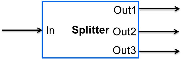
Now you want to develop a new steady-state model of splitter with one input stream and three output streams, as the figure shown below. The splitting factors for the first and second outlets are $k_1$ and $k_2$ respectively.

You need the following steps:

Copy the directory with the template unit <PathToSolution>\ModelsCreatorSDK\UnitsTemplates\SteadyStateUnit to the directory for new units <PathToSolution>\ModelsCreatorSDK\Units\.
Rename the copied template’s directory SteadyStateUnit to MySplitter. Open the directory MySplitter and rename file SteadyState.vcxproj to MySplitter.vcxproj.
Open the template solution <PathToSolution>\ModelsCreatorSDK\Dyssol.sln in Visual Studio.
Add project with your new unit to the solution: select in Visual Studio File → Add → Existing Project and specify path to the project file <PathToSolution>\ModelsCreatorSDK\Units\MySplitter\MySplitter.vcxproj.
Rename added project in Visual Studio from UnitT_SteadyState to Unit_MySplitter.
Open Unit_MySplitter → Unit.cpp in the Visual Studio’s Solution Explorer and extend the unit with the following functionality (please refer to Basic unit, Stream and label-PSD when necessary):

Modify constructor CUnit():
- Specify unit’s name by changing value of variable m_sUnitName to My Splitter. This name will appear in the drop-down list for unit types in Dyssol simulation.
- Specify author’s name by changing value of variable m_sAuthorName.
- Set new unique key of the unit by changing value of variable m_sUniqueID to some random string. To generate such a string GUID generator of Visual Studio can be used Tools → Create GUID.
- Add two additional output ports and rename all of them.
CUnit::CUnit() { // Basic unit's info m_sUnitName = "MySplitter"; m_sAuthorName = "MyName"; m_sUniqueID = "B59F8349A7014AC294D6580C0D8E21FE"; // Add ports AddPort("In", INPUT_PORT); AddPort("Out1", OUTPUT_PORT); AddPort("Out2", OUTPUT_PORT); AddPort("Out3", OUTPUT_PORT); // Add unit parameters - splitting factors AddConstParameter("k1", 0, 1, 0, "k1"); AddConstParameter("k2", 0, 1, 0, "k2"); }
Modify function Initialize(): remove all codes in it.

Modify function Simulate():

Here you should perform all steps which are needed in the simulaition, including get port streams, set mass flow of inlet streams and the calculation of output streams. Also don’t forget to give user warning if some streams becomes minus.

void CUnit::Simulate(double _dTime) {

// Get streams of all ports and assign them to corresponding material streams
CMaterialStream* pInStream = GetPortStream("In");
CMaterialStream* pOutStream1 = GetPortStream("Out1");
CMaterialStream* pOutStream2 = GetPortStream("Out2");
CMaterialStream* pOutStream3 = GetPortStream("Out3");

// Copy inlet stream to all outlet streams
pOutStream1->CopyFromStream(pInStream, _dTime);
pOutStream2->CopyFromStream(pInStream, _dTime);
pOutStream3->CopyFromStream(pInStream, _dTime);

// Set mass flow rate of inlet stream
double dMassFlowIn = pInStream->GetMassFlow(_dTime);

// Add splitting factors
double dSplitFactor1 = GetConstParameterValue("k1");
double dSplitFactor2 = GetConstParameterValue("k2");

// Give warning if sum of splitting factors is greater than 1
if (dSplitFactor1 + dSplitFactor2 > 1)
        RaiseError("Warning about minus outlet 3...");

// Set calculated mass flow rate to corresponding outlet streams
pOutStream1->SetMassFlow(_dTime, dMassFlowIn * dSplitFactor1);
pOutStream2->SetMassFlow(_dTime, dMassFlowIn * dSplitFactor2);
pOutStream3->SetMassFlow(_dTime, dMassFlowIn * (1 - dSplitFactor1 - dSplitFactor2));

}

Perform test simulation:

Now you have your complete code for the splitter. Build the solution and then run Dyssol in debug mode. Add material streams and the unit, choose the unit type “MySplitter”, set inlet mass flow and splitting factors according to the table below, and finally check if the results are correct. Finally, save the simulation file for the example of developing a dynamic unit.

General

Materials

Sand

Phases

Solid

Inlet

Time points

0 s

Mass stream

1 kg/s

Phase mass fractions

Solid: 1

Compounds mass fractions

Sand: 1

Options

Simulation time

60 s

Development of steady-state units with internal non-linear solver

You can solve nonlinear equation systems automatically in Dyssol system. In this case, the unit should contain one or several additional objects of CNLModel class. This class is used to describe non-linear systems and can be automatically solved with CNLSolver class.

Unit::Unit()

Constructor of the unit: called only once when unit is added to the flowsheet. In this function a set of parameters should be specified:

Basic info:
- m_sUnitName: Name of the unit that will be displayed in Dyssol.
- m_sAuthorName: Unit’s author
- m_sUniqueID: Unique identificator of the unit. Simulation environment distinguishes different units with the help of this identificator.
You must ensure that ID of your unit is unique. This ID can be created manually or using GUID-generator of Visual Studio (Tools → GUID Genarator).
Specify ports for stream in- and outlet(s): add new, rename or delete existing.
Additional internal material streams can be defined here.
Sepcify unit parameters.
All other operations, which should take place only once during the unit’s creation.

Unit::~Unit()

Destructor of the unit: called only once when unit is removed from the flowsheet. Here all memory which has been previously allocated in the constructor should be freed.

Unit::Initialize(double _dTime)

Unit‘s initialization. This function is called only once at the start of the simulation at time point dTime. Starting from this point, information about defined compounds, phases, distributions, etc. are available for the unit. Here you can create state variables and initialize some additionaly objects (for example holdups, material streams, state variables or plots).

In this function, variables of all NLModels should be specified by using function NLModel::AddNLVariable(); connection between NLModel and NLSolver classes should be created by calling function NLSolver::SetModel().

Unit::Simulate(double _dTime)

Steady-state calculation for a specified time point dTime. This function is called iteratively for all time points for which this unit should be calculated. All main calculations should be implemented here. Calculation of the defined NL-system can be run here by calling function NLSolver::Calculate().

Unit::SaveState()

For flowsheets containing recycled streams, SaveState() function is called when the convergence on the current time interval is reached, this also ensures the return to the previous state of the unit if convergence fails during the calculation. Here all internal time-dependent variables which weren’t added to the unit by using AddStateVariable and AddMaterialStream functions should be manually saved. Implementation of this function is not obligatory and can be skipped.

Unit::LoadState()

Load last state of the unit which has been saved with SaveState() function. Implementation of this function is not obligatory and can be skipped.

Unit::Finalize()

Unit‘s finalization. This function is called only once at the end of the simulation. Here one can perform closing and cleaning operations to prepare for the next possible simulation run. Implementation of this function is not obligatory and can be skipped.

NLModel::CalculateFunctions(double* _pVars, double* _pFunc, void* _pUserData)

Here the non-linear system should be specified. This function will be called by solver automatically.

NLModel::ResultsHandler(double _dTime, double* _pVars, void* pUserData)

Handling of results, which are returned from NLSolver on each time point. Called by solver every time when the solution in a new time point is ready.

Application example

In this example, you need to develop a steady-state unit for a simple air classifying process, which separates particles according to their sinking velocity in a fluid stream. Additionally, the time and particle size dependence of separation efficiency should be plotted.

The separation depends on the relative velocity between the fluid and the particles $v_{rel,i} = u_G - v_{P,i}$ . Floating particles with no velocity, i.e. $v_{rel,i} = u_G$ , will be divided evenly to coarse and fines stream.

The separation efficiency and cut-off velocity are defined as in the formulas below.

$\xi_{C,i} = 1 / \left( 1 + \dfrac{w_{cut}}{v_{rel,i}} \cdot e^{x \left[ 1 - \left(\dfrac{v_{rel,i}}{w_{cut}}\right)^3 \right]} \right)$

$w_{cut} = u_G = \dfrac{\dot{m}_G}{\rho_G \cdot A}$

To complete the simulation, you need to solve the following implicit equation system:

$Re_{P,i} = \dfrac{|v_{rel,i}|\cdot d_{P,i}\cdot \rho_G}{\eta_G}$

$C_{W,P,i} = \dfrac{24}{Re_{P,i}} + \dfrac{4}{\sqrt{Re_{P,i}}} + 0.4$

$v_{rel,i} = \sqrt{\dfrac{4\,\rho_P\,d_{P,i}\,g}{3\,\rho_G\,C_{W,P,i}}}$

Note

Notations:

$v_{rel,i}$ – Relative velocity of particle of size class $i$ [m/s]

$v_{P,i}$ – Velocity of particle of size class $i$ [m/s]

$u_G$ – Velocity of gas [m/s]

$\xi_{C,i}$ – Separation efficiency of size class $i$ [-]

$w_{cut}$ – Cut-off velocity [m/s]

$\dot{m}_G$ – Gas mass flow [kg/s]

$Re_{P,i}$ – Reynolds number of size class $i$ [-]

$d_{P,i}$ – Particle diameter of size class $i$ [m]

$C_{W,P,i}$ – Drag coefficient of size class $i$ [-]

$\rho_G$ – Gas density [ $kg/m^3$ ]

$\rho_P$ – Particle / solid density [ $kg/m^3$ ]

$\eta_G$ – Gas dynamic viscosity [Pa·s]

$x$ – Sharpness factor [-]

$A$ – Cross-sectional area [ $m^2$ ]

$g$ – Gravitational acceleration [ $m/s^2$ ]

Now you need the following steps:

Copy the directory with the template unit <PathToSolution>\ModelsCreatorSDK\UnitsTemplates\SteadyStateWithNLSolver\ to the directory for new units <PathToSolution>\ModelsCreatorSDK\Units\. Rename the folder to AirClassifierTemplate and the file SteadyStateWithNLSolver.vcxproj to AirClassifier.vcxproj.
Along with this application example, you obtain a pre-configured template folder of the air classifier unit ...\Task8\AirClassifierTemplate\, in which you find the source file Unit.cpp and header file Unit.h. Copy the contents of them to the corresponding Unit.cpp and Unit.h files in your template folder <PathToSolution>\ModelsCreatorSDK\Units\AirClassifierTemplate\.
Open the template solution <PathToSolution>\ModelsCreatorSDK\Dyssol.sln in Visual Studio.
Add project with your new unit to the solution: select File → Add → Existing Project and specify path to the project file <PathToSolution>\ModelsCreatorSDK\Units\AirClassifierTemplate\. Rename the unit to Unit_AirClassifier.
Open Unit_AirClassifier → Unit.cpp in the Visual Studio’s and extend the unit with the following functionality:

Edit the unit CUnit:

Modify constructor CUnit():
Specify unit’s name by changing value of variable m_sUnitName to Air classifier. This name will appear in the drop-down list for unit types in Dyssol simulation.

Specify author’s name by changing value of variable m_sAuthorName.

For m_sUniqueID, unlike the examples in steady-state unit, DO NOT change the ID, because the given ID is connected with the simulation file provided. If you change the ID, the parameter in simulation file would not be read by Dyssol and you can’t carry out your simulaiton.

Add 2 unit parameters using function AddConstParameter: the cross-sectional area A ranging between 0.01 and 100, and the sharpness factor x ranging between 0.01 and 10. You can set inital value to 1 for both parameters.

You find the example code below:
CUnit::CUnit() {

        // Basic unit's info
        m_sUnitName = "Air classifier";
        m_sAuthorName = "Your name";
        m_sUniqueID = "211D0E54C80A4F3EB464671EEA222932"; // DO NOT change this ID

        // Add ports
        AddPort("Input", INPUT_PORT);
        AddPort("Coarse", OUTPUT_PORT);
        AddPort("Fines", OUTPUT_PORT);

        // Add unit parameters
        AddConstParameter("A", 0.01, 100, 1, "Area"); // A
        AddConstParameter("x", 0.01, 10, 1, "Sharpness"); // x

        // Add user data to model
        m_NLModel.SetUserData(this);

}
Modify function Initialize():
Get the number of size classes (GetClassesNumber(DISTR_SIZE)) and save them to variable num_classes.

For each particle size class add a non-linear variable to the model (AddNLVariable) with initial value 1 and no constraints.

Add a plot to the unit for the separation efficiency: Separation (Y axis is “Separation”) against diameter (X axis is “Diameter”) and time (Z axis is “Time”).

The finished code of the function is shown below.
void CUnit::Initialize(double _dTime) {

        // Check Simulation Setup
        if (!IsPhaseDefined(SOA_VAPOR)) {
                RaiseError("Gas phase not defined."); // Check for gas phase
        }
        if (!IsPhaseDefined(SOA_SOLID)) {
                RaiseError("Solid phase not defined."); // Check for solid phase
        }
        if (!IsDistributionDefined(DISTR_SIZE)) {
                RaiseError("Particle size distribution not defined."); // Check for size distribution
        }

        // Clear all state variables in model
        m_NLModel.ClearVariables();

        // Get number of diameter classes
        unsigned num_classes = GetClassesNumber(DISTR_SIZE);

        // Add variable to the model of nonlinear equation system
        for(unsigned i = 0; i < num_classes; ++i) {
                m_NLModel.AddNLVariable(1.0, 0.0);
                // v_rel_i (relative velocity for each particle size class)
        }

        // Set model to the solver
        if (!m_NLSolver.SetModel(&m_NLModel)) {
                RaiseError(m_NLSolver.GetError());
        }

        // Add Plot
        AddPlot("Plot", "Diameter", "Separation", "Time");

}

Edit the solver CMyNLModel:

Implement function CalculateFunctions(double* _pVars, double* _pFunc, void* _pUserData): in this funciton, the updated values _pFunc of the non-linear variables _pVars is computed until the residual between _pFunc and _pVar reaches a certain tolerance.

Get pointer to the output streams to enable calculation with stream properties.
Get vector with particle diameters (GetClassesMeans(DISTR_SIZE)) and store them to variable d.
Get gas properties (GetPhaseTPDProp() for DENSITY and VISCOSITY) at the time point time.
Save current values of _pVars and save them to variable v_rel.
Calculate variables Re_i, Cwp_i, v_rel_update_i according to the equation system described above and save the value of the relative velocity to _pFunc.

The example code for this function looks like this:

void CMyNLModel::CalculateFunctions(double* _pVars, double* _pFunc, void* _pUserData) {

        // Get pointer to air classifier unit
        auto unit = static_cast<CUnit*>(_pUserData);

        // Get pointers to streams
        CMaterialStream* inStream = unit->GetPortStream("Input");
        CMaterialStream* outStreamC = unit->GetPortStream("Coarse");
        CMaterialStream* outStreamF = unit->GetPortStream("Fines");

        // Overall parameter

        double g = 9.81; // graviational acceleration
        // Get diameter classes and their number
        unsigned num_classes = unit->GetClassesNumber(DISTR_SIZE);
        std::vector<double> d = unit->GetClassesMeans(DISTR_SIZE);

        // Get stream parameters
        double rho_solid = inStream->GetPhaseTPDProp(time, DENSITY, SOA_SOLID);
        double rho_gas = inStream->GetPhaseTPDProp(time, DENSITY, SOA_VAPOR);
        double eta_gas = inStream->GetPhaseTPDProp(time, VISCOSITY, SOA_VAPOR);

        // Get value of variables (v_rel_i) at current iteration of solver
        std::vector<double> v_rel;
        for (unsigned i = 0; i < num_classes; ++i) {
                v_rel.push_back(_pVars[i]);
        }

        // Calculation of new function values of relative velocity
        for (unsigned i = 0; i < num_classes; ++i) {
                // Reynolds number of particle classes Re_i
                double Re_i = (fabs(v_rel[i]) * d[i] * rho_gas) / eta_gas;
                // Drag coefficient of particle classes Cwp_i
                double Cwp_i = 24. / Re_i + 4. / std::sqrt(Re_i) + 0.4;
                // Relative velocity
                double v_rel_update_i = sqrt((4. * rho_solid * d[i] * g) / (3. * rho_gas * Cwp_i));
                // Update function value
                _pFunc[i] = v_rel_update_i;
        }
}

Implement function ResultsHandler(double _dTime, double* _pVars, void* _pUserData): this function processes the results returned by the solver, after convergence is reached.

Initialize output streams for fines by copying the information from input and afterwards setting the total mass flows to zero.
Get unit parameters for A and x (GetConstParameterValue).
Get stream properties from input stream: solid and gas mass flows (GetPhaseMassFlow) as well as particle size distribution (GetPSD).
Calculate cut-velocity w_cut according to the equation for it.
Caculate the separation to the coarse stream xiC_i:
- Save the value of the relative velocity to v_rel_i.
- Calculate xiC_i according to the equation for it.
- Calculate the accumulated mass fraction of coarse stream by adding up xiC_i multiplied by incoming mass fraction of class $i$ , wIn[i].
- Update the Transformation matrices.
- Save xiC_i to vector for later plotting purposes.
Apply transformation matrices to output streams and set the phase mass flows. You need 2 matrices, one for coarse stream and the other for fine stream. Please also notice that all gases must leave with fine stream.

The matrices contain the separatiom efficiency xiC_i of all size classes $i$ .

TInputToCoarse: all elements NOT on diagonal are zero. xiC_i of classe $i$ locates at position $(i,i)$ .

TInputToFine: all elements NOT on diagonal are zero. 1 - xiC_i of classe $i$ locates at position $(i,i)$ .
Plotting: Add a new curve to the plot (AddCurveOnPlot) at time _dTime and then add the points for separation (AddPointOnCurve).

You can find the example code for this function below:

void CMyNLModel::ResultsHandler(double _dTime, double* _pVars, void* _pUserData) {

        // Get pointer to air classifier unit
        auto unit = static_cast<CUnit*>(_pUserData);

        // Get pointers to streams
        CMaterialStream* inStream = unit->GetPortStream("Input");
        CMaterialStream* outStreamC = unit->GetPortStream("Coarse");
        CMaterialStream* outStreamF = unit->GetPortStream("Fines");

        // Get diameter classes and their number
        std::vector<double> d = unit->GetClassesMeans(DISTR_SIZE);
        unsigned num_classes = unit->GetClassesNumber(DISTR_SIZE);

        // Initialize output streams:
        // Setting total mass flow to zero allows only for ...
        // ... setting phase mass flows at the end of the unit
        // (total mass flow will be calculated automatically)
        outStreamC->CopyFromStream(inStream, _dTime);
        outStreamC->SetMassFlow(_dTime, 0);
        outStreamF->CopyFromStream(inStream, _dTime);
        outStreamF->SetMassFlow(_dTime, 0);

        // Setup transformation matrices
        CTransformMatrix TInputToCoarse(DISTR_SIZE, num_classes);
        CTransformMatrix TInputToFines(DISTR_SIZE, num_classes);

        // Get parameters
        double A = unit->GetConstParameterValue("A");
        double x = unit->GetConstParameterValue("x");

        // Get stream parameters
        double dm_solid = inStream->GetPhaseMassFlow(_dTime, SOA_SOLID);
        double rho_solid = inStream->GetPhaseTPDProp(_dTime, DENSITY, SOA_SOLID);
        double dm_gas = inStream->GetPhaseMassFlow(_dTime, SOA_VAPOR);
        double rho_gas = inStream->GetPhaseTPDProp(_dTime, DENSITY, SOA_VAPOR);
        std::vector<double> wIn = inStream->GetPSD(_dTime, PSD_MassFrac);

        // Calculate cut velocity
        double w_cut = dm_gas / (rho_gas * A);

        // Calculate separation efficiency:
        // Fraction of mass in coarse stream
        double wC_acc = 0;
        // Separation efficiency for each particle class
        std::vector<double> xiC;
        for (unsigned i = 0; i < num_classes; ++i) {
                // Get value of variables (v_rel_i) after convergence of solver
                double v_rel_i = _pVars[i];
                // Temporary value for separation of particle class to coarse stream
                double xiC_i;
                // Check values of relative velocity:
                // If v_rel_i < 0, particles are faster than fluid, i.e. they will go to fines
                // Else calculate separation based on functions
                if (v_rel_i < 0) {
                        xiC_i = 0;
                }
                else {
                        double temp_exp = exp( x * (1 - pow(v_rel_i / w_cut, 3)));
                        xiC_i = 1. / (1 + w_cut / v_rel_i * temp_exp);
                }

                // Update fraction of mass that goes to coarse stream
                wC_acc += wIn[i] * xiC_i;
                // Update transformation matrices of the separation
                TInputToCoarse.SetValue(i, i, xiC_i);
                TInputToFines.SetValue(i, i, 1 - xiC_i);
                // Save temporary separation value to vector
                xiC.push_back(xiC_i);
        }

        // Set properties of coarse stream:
        // Apply transformation matrix to coarse stream
        outStreamC->ApplyTM(_dTime, TInputToCoarse);
        // Set coarse solid mass flow
        outStreamC->SetPhaseMassFlow(_dTime, SOA_SOLID, wC_acc * dm_solid);

        // Set properties of fine stream:
        // Apply tranformation matrix to fines stream
        outStreamF->ApplyTM(_dTime, TInputToFines);
        // Set gas mass flow
        outStreamF->SetPhaseMassFlow(_dTime, SOA_VAPOR, dm_gas);
        // Set solid mass flow
        outStreamF->SetPhaseMassFlow(_dTime, SOA_SOLID, (1 - wC_acc) * dm_solid);

        // Plotting separation efficiency for coarse stream
        unit->AddCurveOnPlot("Plot", _dTime);
        unit->AddPointOnCurve("Plot", _dTime, d, xiC);

}

Test the unit in Dyssol:

Build the solution and run Dyssol: Build → Build Solution, and then Debug → Start Debugging.
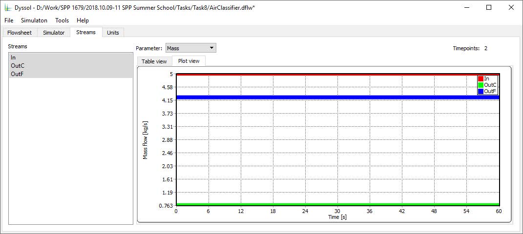
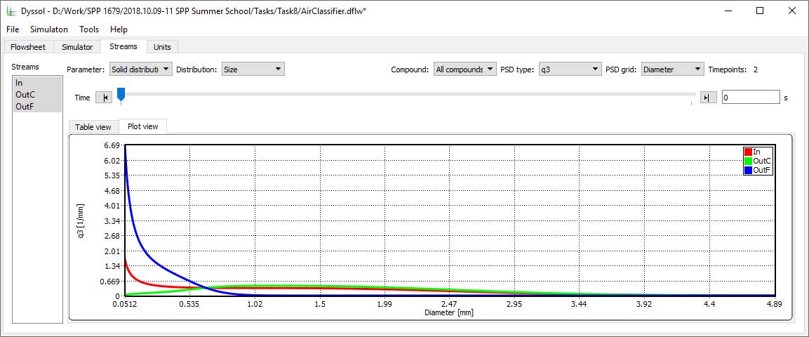
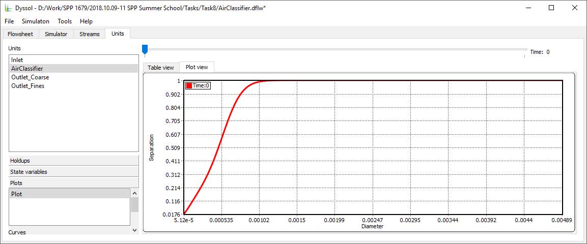
Use exemplary flowsheet ...\Tasks8\AirClassifier.dflw to test your unit. Compare your results with the expected ones below.

Development of dynamic units

Unit::Unit()

Constructor of the unit: called only once when unit is added to the flowsheet. In this function a set of parameters should be specified:

Basic info:
- m_sUnitName: Name of the unit that will be displayed in Dyssol.
- m_sAuthorName: Unit’s author
- m_sUniqueID: Unique identificator of the unit. Simulation environment distinguishes different units with the help of this identificator. You must ensure that ID of your unit is unique. This ID can be created manually or using GUID-generator of Visual Studio (Tools → GUID Genarator).
Specify ports for stream in- and outlet(s): add new, rename or delete existing.
Specify unit parameters.
Define internal holdups and additional material streams.
Define all other operations, which should take place only once during the unit’s creation.

Unit::~Unit()

Destructor of the unit: called only once when unit is removed from the flowsheet. Here all memory which has been previously allocated in the constructor should be freed.

Unit::Initialize(double _dTime)

Unit‘s initialization. This function is called only once at the start of the simulation at dTime. Starting from this point, information about defined compounds, phases, distributions, etc. are available for the unit. Here you can create state variables and initialize some additionaly objects (e.g. holdups, material streams or state variables).

Unit::Simulate(double _dStartTime, double _dEndTime)

Dynamic calculation of the unit on a specified time interval from dStartTime to dEndTime. All logic of the unit’s model must be implemented here.

Unit::SaveState()

For flowsheets containing recycled streams, SaveState() function is called when the convergence on the current time interval is reached, this also ensures the return to the previous state of the unit if convergence fails during the calculation. Here all internal time-dependent variables which weren’t added to the unit by using AddStateVariable, AddMaterialStream or AddHoldup functions should be manually saved. Implementation of this function is not obligatory and can be skipped.

Unit::LoadState()

Load last state of the unit which has been saved with the SaveState() function. Implementation of this function is not obligatory and can be skipped.

Unit::Finalize()

Unit‘s finalization. This function is called only once at the end of the simulation. Here one can perform closing and cleaning operations to prepare for the next possible simulation run. Implementation of this function is not obligatory and can be skipped.

Application example

You will learn to implement a simple dynamic unit (however without any physical meaning), where the basic functionality of classes CBaseUnit, CMaterialStream and CHoldup can be tested.

Do the following steps:

Copy a directory with the template unit <PathToSolution>\ModelsCreatorSDK\UnitsTemplates\DynamicUnit to the directory for new units <PathToSolution>\ModelsCreatorSDK\Units\.
Rename the copied template’s directory DynamicUnit to Basics. Open the directory Basics and rename the file Dynamic.vcxproj` to Basics.vcxproj.
Open the template solution (<PathToSolution>\Dyssol.sln) in Visual Studio.
Add project with your new unit to the solution: select in Visual Studio File → Add → Existing Project and specify path to the project file <PathToSolution>\ModelsCreatorSDK\Units\Basics\Basics.vcxproj.
Rename added project in Visual Studio from UnitT_Dynamic to Unit_Basics.
Open Unit_Basics → Unit.cpp in the Visual Studio’s Solution Explorer and develop your unit as shown follows. You can use Basic unit, Stream and label-PSD for references.

Modify constructor CUnit():

Specify unit’s name by changing value of variable m_sUnitName to Basics. This name will appear in the drop-down list for unit types in Dyssol simulation.

Specify author’s name by changing value of variable m_sAuthorName.

Set new unique key of the unit by changing value of variable m_sUniqueID to some random string. To generate such a string, you can use GUID generator of Visual Studio (Tools → Create GUID).

Now your code for constructor should look like this:
CUnit::CUnit() {

        // Basic unit's info
        m_sUnitName = "Basics";
        m_sAuthorName = "Your name";
        m_sUniqueID = "30D8887B8E5F4BF5B91B98342684E707";

        // Add ports
        AddPort("InPort", INPUT_PORT);
        AddPort("OutPort", OUTPUT_PORT);

        // Add unit parameters
        AddTDParameter("ParamTD", 0, 1e+6, 0, "Unit parameter description");
        AddConstParameter("ParamConst", 0, 1e+6, 0, "Unit parameter description");
        AddStringParameter("ParamString", "Initial value", "Unit parameter description");

        // Add holdups
        AddHoldup("HoldupName");

}

Modify function Initialize(double _dTime):

Add warnings if liquid or vapor phases are not defined. Use functions IsPhaseDefined and RaiseWarning.

Add an internal material stream named “BufStream” using the function AddMaterialStream.

Add new plot with the name “Plot1” to show dependency of holdup’s mass (Y axis is “Mass”) over time (X axis is “Time”). Add a curve on this plot with the name “Curve1”. Use the functions AddPlot and AddCurveOnPlot.

An example for this section is shown below.
void CUnit::Initialize(double _dTime) {

        /// Add state variables ///
        AddStateVariable("VarName", 0, true);
        if (!IsPhaseDefined(SOA_LIQUID)) {
                RaiseWarning("Liquid phase has not been defined");
        }
        if (!IsPhaseDefined(SOA_VAPOR)) {
                RaiseWarning("Vapor phase has not been defined");
        }

        // Add buffer stream
        AddMaterialStream("BufStream");

        // Add plot
        AddPlot("Plot1", "Mass", "Time");
        AddCurveOnPlot("Plot1", "Curve1");

}

Modify funciton Simulate(double _dStartTime, double _dEndTime):

Obtain pointer to the BufStream into the new variable CMaterialStream *bufStream (with the function GetMaterialStream).
Add new time point _dStartTime to BufStream with bufStream->AddTimePoint.
Copy inlet into BufStream at _dEndTime with the function bufStream->CopyFromStream.
Set mass flow to 12.5 kg/s of the liquid phase in BufStream at t = 10s (bufStream->SetPhaseMassFlow).
Add inlet to the holdup on entire time interval from _dStartTime to _dEndTime (pHoldup->AddStream).
Copy the holdup into the outlet for _dStartTime time point with mass flow 1 kg/s (pOutStream->CopyFromHoldup).
Set new temperature T = 320 K to the outlet at t = 15 s (pOutStream->SetTemperature).
Plot mass of the holdup for all defined time points. Use the functions GetAllDefinedTimePoints, AddPointOnCurve and pHoldup->GetMass.

The example code looks like follows:

void CUnit::Simulate(double _dStartTime, double _dEndTime) {

        // Get pointers to streams
        CMaterialStream* pInStream = GetPortStream("InPort");
        CMaterialStream* pOutStream = GetPortStream("OutPort");
        CMaterialStream* bufStream = GetMaterialStream("bufStream");

        // Get pointers to holdups
        CHoldup* pHoldup = GetHoldup("Holdup");

        // Add start time point to bufStream
        bufStream->AddTimePoint(_dStartTime);

        // Copy inlet stream into bufStream
        bufStream->CopyFromStream(pInStream, _dEndTime);

        // Set mass flow 12.5 kg/s of liquid phase in bufStream at time point 10 s
        bufStream->SetPhaseMassFlow(10, SOA_LIQUID, 12.5, BASIS_MASS);

        // Add inlet to the holdup on entire time interval
        pHoldup->AddStream(pInStream, _dStartTime, _dEndTime);

        // Copy the holdup into outlet stream at end time point with mass flow 1 kg/s
        pOutStream->CopyFromHoldup(pHoldup, _dStartTime, 1);

        // Set new temperature 320 K to outlet at time point 15 s
        pOutStream->SetTemperature(15, 320);

        // Plot holdup mass for all defined time points
        std::vector<double> times = GetAllDefinedTimePoints(_dStartTime, _dEndTime);
        for (int i = 0; i < times.size(); i++) {
                double x = times[i];
                double y = pHoldup->GetMass(times[i], BASIS_MASS);
                AddPointOnCurve("Time dependence of holdup mass", "Curve1", x, y);
        }

        // Data acquisition:
        // Get unit parameters
        double TDParameter = GetTDParameterValue("ParamTD", 5);
        double ConstParameter = GetConstParameterValue("ParamConst");
        std::string StringParameter = GetStringParameterValue("ParamString");
        // Get common compound information
        std::vector<std::string> compounds = GetCompoundsList(); //only one compound in task6, so only one element in compounds array
        double molarMass = GetCompoundConstant(compounds[0], MOLAR_MASS);
        double critTemp = GetCompoundConstant(compounds[0], CRITICAL_TEMPERATURE);
        double density = GetCompoundTPDProp(compounds[0], DENSITY, 273, 1e5);
        // Get tolerance
        double absTol = GetAbsTolerance();
        double relTol = GetRelTolerance();
        // Get overall properties of streams and holdups
        double massFlow = pInStream->GetMassFlow(2, BASIS_MASS);
        double massHoldup = pHoldup->GetMass(5, BASIS_MASS);
        double outTemp = pOutStream->GetTemperature(15);
        double molarMassHoldup = pHoldup->GetOverallProperty(1, MOLAR_MASS);
        // Get solid distribution information
        std::vector<double> PSD_b3 = pHoldup->GetPSD(50, PSD_Q3);
        std::vector<double> PSD_s3 = pHoldup->GetPSD(50, PSD_q3);

}

Test your unit in Dyssol:
- Build the solution by Build → Build Solution and run Dyssol by Debug → Start Debugging.
  Change the flowsheet from example of steady-state unit to be able to test new unit: remove units Out2, Out3 and streams Out2, Out3.
  
  Change unit model MySplitter to Basics. Set unit parameters as ParamTD = 1.2, ParamConst = 1e-8.
  
  Run the simulation, make sure the simulation is finished and save the obtained flowsheet as Task6. Close Dyssol.
Extend the Simulate function with the code to obtain values of unit’s and streams’ parameters, which are specified in the table at the end of this section.

Use breakpoints in debug mode of Visual Studio to obtain values of variables at runtime. To do this, place a breakpoint at the end of the function Simulate (select desired line of code, then choose Debug → Toggle Breakpoint or press F9) and start debugging (Debug → Start Debugging or F5). After pressing the Simulate button in Dyssol, the program stops at the breakpoint. Values of all previously calculated variables will be available on mouse hover in Visual Studio. Compare your results with expected values below.

Unit parameters:

Parameter

Function

Expected value

Value of Time-dependent unit parameter ParamTD at time point 5s

GetTDParameterValue()

1.2

Value of constant unit parameter ParamConst

GetConstParameterValue()

1E-8

Value of string unit parameter ParamString

GetStringParameterValue()

Initial value

Common compounds information:

Parameter

Function

Expected value

List of defined compounds

GetCompoundsList()

4031BC62EC7F17EFA33F

Molar mass of the first defined compound

GetCompoundConstant(… MOLAR_MASS)

0.06

Critical temperature of the first defined compound

GetCompoundConstant(… CRITICAL_TEMPERATURE)

3500

Density of the first compound by T = 273 K, P = 1e+5 Pa

GetCompoundTPDProp(… DENSITY, …)

1600

Tolerances:

Parameter

Function

Expected value

Global absolute tolerance

GetAbsTolerance()

1E-6

Global relative tolerance

GetRelTolerance()

0.001
Overall properties of streams and holdups:
Parameter

Function

Expected value

Mass flow of the inlet at t = 2 s

pInStream->GetMassFlow()

1

Mass of the holdup at t = 5 s

pHoldup->GetMass()

5

Temperature of the outlet at t = 15 s

pOutStream->GetTemperature()

300

Molar mass of the holdup at t = 1 s

pHoldup->GetOverallProperty()

0.06
Note

You will see the outlet temperature at 15 s is not changed to 320 K. In this process, only _dStartTime and _dEndTime are defined in the simulation (due to the simulation file of a steady-state process), the time point t = 15 s is not defined and thus no change will take place. If you add a time point for the outlet stream,
pOutStream->AddTimePoint(15);
the temperature will change to 320 K at t = 15 s.

Therefore, please pay attention to your time points during the dynamic simulation. A time point must be defined in advance, at which your simulation is performed. However, in most cases, the time points during a simulation are calculated by the solvers and you don’t need to define them extra.
Note

You can also observe the temperature change at _dEndTime to 320 K, like the code below:
pOutStream->CopyFromHoldup(pHoldup, _dStartTime, 1);
pOutStream->SetTemperature(_dEndTime, 320);
// ... intermediate code ... //
double outTemp = pOutStream->GetTemperature(_dEndTime);
In this case, the outlet temperature is still 300 K. The reason is that the default value of variable DeleteDataAfter in CopyFromHoldup is true, which means the information at copied time (here _dStartTime) is kept and those afterwards are deleted. Since there is no information at _dEndTime, the program returns the temperature at _dStartTime.

If you set the value of variable DeleteDataAfter to false, the outlet temperature doesn’t change either, because only the holdup information at _dStartTime is copied, which has nothing to do with that at _dEndTime. You must also copy the holdup info at the end in order to change the temperature at the end.
pOutStream->CopyFromHoldup(pHoldup, _dStartTime, 1, false);
pOutStream->CopyFromHoldup(pHoldup, _dEndTime, 1);
pOutStream->SetTemperature(_dEndTime, 320);
// ... intermediate code ... //
double outTemp = pOutStream->GetTemperature(_dEndTime);
For developing dynamic units in Dyssol, don’t forget to treat your parameter at different time points separately.
Solid distributed properties and PSD of streams and holdups:

Parameter

Function

Expected value

$Q_3$ distribution of the holdup at t = 50 s

pHoldup->GetPSD(… PSD_Q3)

(not applicable)

$q_3$ distribution of the holdup at t = 50 s

pHoldup->GetPSD(… PSD_q3)

(not applicable)

Development of dynamic units with internal DAE solver

You can solve systems of DAE automatically in Dyssol system. In this case, the unit should contain one or several additional objects of CDAEModel class. This class is used to describe DAE systems and can be automatically solved by class CDAESolver.

Unit::Unit()

Constructor of the unit: called only once when unit is added to the flowsheet. In this function a set of parameters should be specified:

Basic info:
- m_sUnitName: Name of the unit that will be displayed in Dyssol.
- m_sAuthorName: Unit’s author.
- m_sUniqueID: Unique identificator of the unit. Simulation environment distinguishes different units with the help of this identificator. You must ensure that ID of your unit is unique. This ID can be created manually or using GUID-generator of Visual Studio (Tools → GUID Genarator).
Specify ports: add new, rename or delete existing.
If unit has some additionally parameters, than specify them here.
Internal holdups and additional material streams can be defined here.
All other operations, which should take place only once during the unit’s creation.

Unit::~Unit()

Destructor of the unit: called only once when unit is removed from the flowsheet. Here all memory which has been previously allocated in the constructor should be freed.

Unit::Initialize(double _dTime)

Unit‘s initialization. This function is called only once at the start of the simulation. Starting from this point, information about defined compounds, phases, distributions, etc. are available for the unit. Here you can create state variables and initialize some additionaly objects (e.g. holdups, material streams or state variables).

In this function, variables of all DAEModels should be specified by using function AddDAEVariable; connection between CDAEModel and CDAESolver classes should be created by calling function SetModel.

Unit::Simulate(double _dStartTime, double _dEndTime)

Dynamic calculation for a specified time interval. Is called for each time window on simulation interval. Calculation of the defined DAE-system can be run here by calling function DAESolver::Calculate().

Unit::SaveState()

For flowsheets containing recycled streams, SaveState() function is called when the convergence on the current time interval is reached, this also ensures the return to the previous state of the unit if convergence fails during the calculation. Here all internal time-dependent variables which weren’t added to the unit by using AddStateVariable, AddMaterialStream or AddHoldup functions should be manually saved. Implementation of this function is not obligatory and can be skipped.

Unit::LoadState()

Load last state of the unit which has been saved with SaveState() function. Implementation of this function is not obligatory and can be skipped.

Unit::Finalize()

Unit‘s finalization. This function is called only once at the end of the simulation. Here one can perform closing and cleaning operations to prepare for the next possible simulation run. Implementation of this function is not obligatory and can be skipped.

DAEModel::CalculateResiduals(double _dTime, double* _pVars, double* _pDers, double* _pRes, void* _pUserData)

Here the DAE system should be specified in implicit form. This function will be called by solver automatically.

DAEModel::ResultsHandler(double _dTime, double* _pVars, double* _pDers, void* _pUserData)

Handling of results, which are returned from DAESolver on each time point. Called by solver every time when the solution in a new time point is ready.

Application example

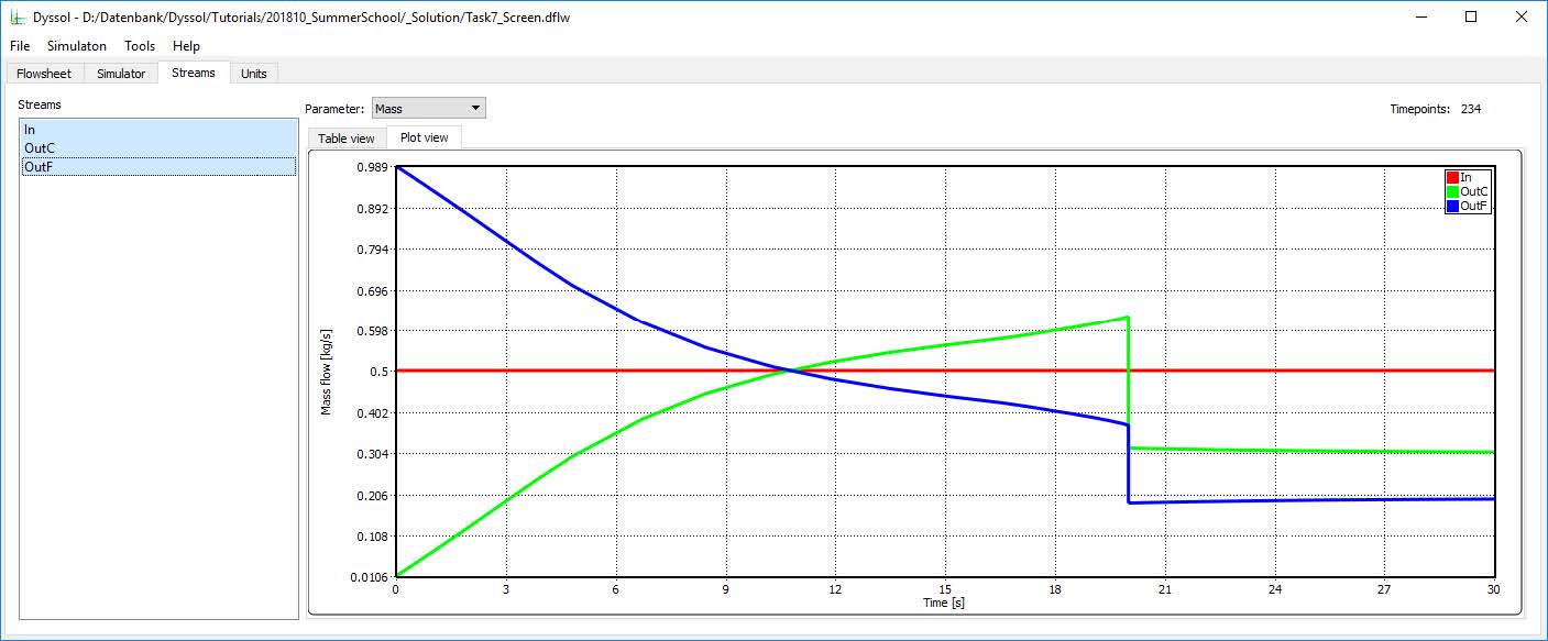
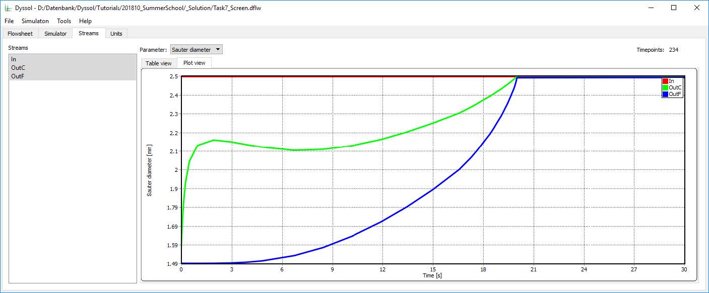
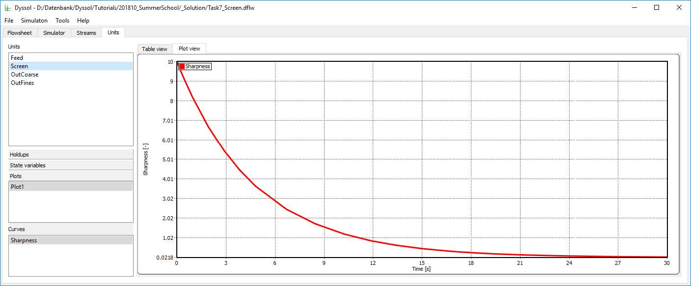
In this example, you will learn how to develop a dynamic screen model with a holdup, wherein the screening efficiency reduces with time and also depends on the holdup‘s mass. Additionally, the time dependency of screening efficiency should be plotted.

The screening efficiency is calculated according to the equation below:

$G(x_i) = \left [ 1 + \left( \dfrac{x_{cut}}{x_i} \right )^2 \cdot e^{\alpha \cdot \left( 1 - (x_i / x_{cut})^2 \right ) } \right ]^{-1}$

To complete the simulation, you need to solve the following dynamic equation system:

$\dot{m}_c + \dot{m}_f = \begin{cases} \dot{m}_{out} & \text{sufficient holdup mass} \\ \dot{m}_{in} & \text{insufficient holdup mass} \\ \end{cases}$

$\dfrac{dM_h}{dt} = \dot{m}_{in} - \dot{m}_{out}$

$\dfrac{d\alpha}{dt} = -\alpha \cdot k_1 - \alpha \cdot M_h \cdot k_2$

Note

Notations:

$\alpha$ – separation sharpness (specified by user)

$x_{cut}$ – cut size (specified by user)

$\dot{m}_{out}$ – output mass flow (specified by user)

$k_1$ – time-dependent sharpness reduction factor [ $s^{-1}$ ] (specified by user)

$k_2$ – mass-dependent sharpness reduction factor [ $kg^{-1}$ ] (specified by user)

$G(x_i)$ – screening efficiency for particle of size class $i$

$\dot{m}_c$ – mass flow of coarse particles

$\dot{m}_f$ – mass flow of fines particles

$\dot{m}_{in}$ – input mass flow

$M_h$ – holdup mass

$x_i$ – particle diameter

Now you need the following steps:

Copy the directory with the template unit <PathToSolution>\ModelsCreatorSDK\UnitsTemplates\DynamicWithDAESolver\ to the directory for new units <PathToSolution>\ModelsCreatorSDK\Units\. Rename the folder to ScreenTemplate and the file DynamicWithDAESolver.vcxproj to Screen.vcxproj.
Along with this application example, you obtain a pre-configured template folder of the air classifier unit ...\Task7\ScreenTemplate\, in which you find the source file Unit.cpp and header file Unit.h. Copy the contents of them to the corresponding Unit.cpp and Unit.h files in your template folder <PathToSolution>\ModelsCreatorSDK\Units\ScreenTemplate\.
Open the template solution <PathToSolution>\ModelsCreatorSDK\Dyssol.sln in Visual Studio.
Add project with your new unit to the solution: select File → Add → Existing Project and specify path to the project file <PathToSolution>\ModelsCreatorSDK\Units\ScreenTemplate\. Rename the unit to Unit_Screen.
Open Unit_AirClassifier → Unit.cpp and extend the unit with the following functionality:

Edit the unit CUnit:

Modify constructor CUnit():
Specify unit’s name by changing value of variable m_sUnitName to Dynamic screen. This name will appear in the drop-down list for unit types in Dyssol simulation.

Specify author’s name by changing the value of the variable m_sAuthorName.

For m_sUniqueID, unlike the examples in steady-state unit, DO NOT change the ID, because the given ID is connected with the simulation file provided. If you change the ID, the parameter in simulation file would not be read by Dyssol and you can’t carry out your simulaiton.

Add unit parameters: add 5 constant unit parameters using AddConstParameter and set their initial values according to your wish:

0 ≤ alpha ≤ 100

0 ≤ Xcut ≤ 1

0 ≤ Mout ≤ 100

0 ≤ k1 ≤1

0 ≤ k2 ≤ 1

Now your constructor code looks like this:
CUnit::CUnit() {

        // Basic unit's info
        m_sUnitName = "Dynamic Screen";
        m_sAuthorName = "Your name";
        m_sUniqueID = "C7755DAF619C448D863D1CBCC13648BC"; // DO NOT change this ID

        // Add ports
        AddPort("Input", INPUT_PORT);
        AddPort("Coarse", OUTPUT_PORT);
        AddPort("Fines", OUTPUT_PORT);

        // Add unit parameters
        AddConstParameter("alpha", 0, 100, 1, "Separation sharpness"); // alpha
        AddConstParameter("Xcut", 0, 1, 0, "Cut size [m]"); // Xcut
        AddConstParameter("Mout", 0, 100, 0, "Output mass flow [kg/s]"); // Mout
        AddConstParameter("k1", 0, 1, 0, "Time-dependent sharpness reduction factor [1/s]"); // k1
        AddConstParameter("k2", 0, 1, 0.001, "Mass-dependent sharpness reduction factor [1/kg]"); // k2

        // Add holdups
        AddHoldup("Holdup");

        // Set this unit as user data of model
        m_Model.SetUserData(this);

}
Modify function Initialize(double _dTime):
Check flowsheet parameters: raise errors (RaiseError) if distribution by size (IsDistributionDefined) and the solid phase (IsPhaseDefined) are not defined.

Add plots: add a plot with the name “Plot1” to show dependency of the separation sharpness (Y axis is “Sharpness”) over time (X axis is “Time”). Add a curve on this plot with the name “Sharpness”. Use functions AddPlot, AddCurveOnPlot.

Add state variables to the model: add differential and algebraic variables (AddDAEVariable), which will be calculated by the internal DAE solver (see equations above). Set all initial values to 0.

Differential variable for the holdup mass Holdup (already defined);

Differential variable for the separation sharpness alpha;

Algebraic variable for the output mass flow Mout.

The example code for this function is shown below.
void CUnit::Initialize(double _dTime) {

        // Check flowsheet parameters
        if (!IsDistributionDefined(DISTR_SIZE)) {
                RaiseError("Size distribution has not been defined!");
        }
        if (!IsPhaseDefined(SOA_SOLID)) {
                RaiseError("Solid phase has not been defined!");
        }

        // Add plots
        AddPlot("Plot1", "Time [s]", "Sharpness [-]");
        AddCurveOnPlot("Plot1", "Sharpness");

        // Clear all state variables in model
        m_Model.ClearVariables();

        // Add state variables to a model
        m_Model.AddDAEVariable(true, GetHoldup("Holdup")->GetMass(_dTime), 0); // holdup mass
        m_Model.AddDAEVariable(true, GetConstParameterValue("alpha"), 0); // separation sharpness
        m_Model.AddDAEVariable(false, GetConstParameterValue("Mout"), 0); // output mass flow

        // Set tolerances to model
        m_Model.SetTolerance(GetRelTolerance() * 10, GetAbsTolerance() * 10);

        // Set model to a solver
        if (!m_Solver.SetModel(&m_Model)) {
                RaiseError(m_Solver.GetError());
        }

}

Edit the solver CMyDAEModel:

Modify function CalculateResiduals(double _dTime, double* _pVars, double* _pDers, double* _pRes, void* _pUserData): this function computes the problem residual for given values of the independent variable _dTime, state vector _pVars (defined variables from 7.3), and their derivatives _pDerivs. Here the DAE system itself must be specified in implicit form.
Get pointers to streams: obtain pointer to holdup for further work with its parameters: GetHoldup.

Get values of input and internal parameters: obtain current values of:

unit parameters $k_1$ , $k_2$ , $\dot{m}_{out}$ (unit->GetConstParameterValue())

mass flow of the inlet at current time point (inStream->GetMassFlow())

mass in the holdup at current time point (holdup->GetMass())

Calculate and set residuals: calculate residuals of all variables from 7.2 according to equations above:

_pVars[0] – calculated value of the holdup mass $M_h$

_pVars[1] – calculated value of the separation sharpness $\alpha$

_pVars[2] – calculated value of the output mass flow $\dot{m}_{out}$ .

The example code is shown below.
void CMyDAEModel::CalculateResiduals(double _dTime, double* _pVars, double* _pDers, double* _pRes, void* _pUserData) {

        // Get pointers to streams
        CUnit *unit = static_cast<CUnit*>(_pUserData);
        CMaterialStream *inStream = unit->GetPortStream("Input"); // Input
        CHoldup *holdup = unit->GetHoldup("Holdup"); // Holdup

        // Get time parameters
        double prevTime = holdup->GetLastTimePoint();
        double dTime = _dTime - prevTime;

        // Get values of input and internal parameters
        double k1 = unit->GetConstParameterValue("k1"); // k1
        double k2 = unit->GetConstParameterValue("k2"); // k2
        double mOut = unit->GetConstParameterValue("Mout"); // Mout
        double mIn = inStream->GetMassFlow(_dTime); // Mass flow in inlet
        double MhPrev = holdup->GetMass(prevTime); // Mass in holdup

        // Calculate and set residuals
        double derMassHoldup = mIn - mOut;
        double derAlpha = (-_pVars[1] * k1 - _pVars[1] * (MhPrev + derMassHoldup)*k2);
        double valMassFlowOut;
        if (mOut * dTime < _pVars[0]) {
                valMassFlowOut = mOut;
        }
        else {
                valMassFlowOut = mIn;
        }

        _pRes[0] = _pDers[0] - derMassHoldup;
        _pRes[1] = _pDers[1] - derAlpha;
        _pRes[2] = _pVars[2] - valMassFlowOut;

}
Modify function ResultsHandler(double _dTime, double* _pVars, double* _pDerivs, void *_pUserData): this function processes the results returned by the solver at each calculated step. Is called by solver every time, when the solution in the new time point is ready.
Get pointers to streams: obtain pointers to streams Input, Coarse and Fines, as well as to holdup Holdup for further work with their parameters (use functions GetPortStream and GetHoldup).

Add points on plot: put value of the separation sharpness $\alpha$ (calculated by the DAE solver in _pVars[1]) on the curve “Sharpness” of the plot “Plot1”. Use the function AddPointOnCurve().

Mix the input stream with the holdup: use the function AddStream to add the content of the inlet between time points holdup->GetLastTimePoint() and _dTime to the holdup.

Calculate transformation matrices: calculate values of the screening efficiency $G(x_i)$ to fill in two transformation matrices:

THoldupToFines – to transform holdup into the output of fines material. All elements NOT on diagonal are zero. $G(x_i)$ of classe $i$ locates at position $(i,i)$ .

THoldupToCoarse – to transform holdup into the output of coarse material. All elements NOT on diagonal are zero. The value $1-G(x_i)$ of classe $i$ locates at position $(i,i)$ .

Here also fractions of mass streams of coarse and fines outlets must be calculated according to the grade efficiency $G(x_i)$ . The screen unit of Plitt’s model can be used as a reference.

Copy the holdup to the output streams: copy all parameters of the holdup into the both outlet streams using function CopyFromHoldup and set their new mass flows, calculated by the DAE solver in _pVars[2]. This calculated mass must be previously scaled according to the grade efficiency $G(x_i)$ .

Apply transformation matrices: apply transformation of the PSD to the outputs, using the function ApplyTM.

Set new mass to the holdup, using the function SetMass. It is calculated by the DAE solver in _pVars[0].

The example code looks like this:
void CMyDAEModel::ResultsHandler(double _dTime,double* _pVars, double* _pDerivs, void *_pUserData) {

        // Get pointers to streams
        CUnit *unit = static_cast<CUnit*>(_pUserData);
        CMaterialStream *inStream = unit->GetPortStream("Input"); // Input
        CMaterialStream *outStreamC = unit->GetPortStream("Coarse"); // Coarse
        CMaterialStream *outStreamF = unit->GetPortStream("Fines"); // Fines
        CHoldup *holdup = unit->GetHoldup("Holdup"); // Holdup

        // Get values of unit parameters at current time point
        double xCut = unit->GetConstParameterValue("Xcut");
        double Mh = _pVars[0];
        double alpha = _pVars[1];
        double mFlowOut = _pVars[2];

        // Add points on plot
        unit->AddPointOnCurve("Plot1", "Sharpness", _dTime, alpha);

        // Mix input stream with holdup
        holdup->AddStream(inStream, holdup->GetLastTimePoint(), _dTime);

        // Obtain parameters for PSD calculation
        unsigned classesNum = unit->GetClassesNumber(DISTR_SIZE);
        std::vector<double> x = unit->GetPSDMeanDiameters();
        std::vector<double> holdupPSD = holdup->GetPSD(_dTime, PSD_MassFrac);

        // Setup transformation matrices
        CTransformMatrix THoldupToCoarse(DISTR_SIZE, classesNum);
        CTransformMatrix THoldupToFines(DISTR_SIZE, classesNum);

        // Calculate transformation matrices
        double massFactor = 0;
        for (unsigned i = 0; i < classesNum; i++) {
                for (unsigned j = 0; j < classesNum; j++) {
                        if (i == j)  { // if this is a diagonal element
                                double val = 1 / (1 + std::pow(xCut / x[i], 2.0) * std::exp(alpha * (1 - (std::pow(x[i] / xCut, 2.0)))));
                                THoldupToCoarse.SetValue(i, j, val);
                                THoldupToFines.SetValue(i, j, 1 - val);
                                massFactor = massFactor + holdupPSD[i] * val;
                        }
                }
        }

        // Copy holdup to output streams
        outStreamC->CopyFromHoldup(holdup, _dTime, mFlowOut*massFactor);
        outStreamF->CopyFromHoldup(holdup, _dTime, mFlowOut*(1 - massFactor));

        // Apply transformation matrix
        outStreamC->ApplyTM(_dTime, THoldupToCoarse);
        outStreamF->ApplyTM(_dTime, THoldupToFines);

        // Set new mass to the holdup
        holdup->SetMass(_dTime, Mh);

}

Test your unit in Dyssol:

Build the solution and run Dyssol: Build → Build Solution, and then Debug → Start Debugging.
Use exemplary flowsheet ...\Task7\DynamicScreen.dflw to test your unit. Compare your results with the expected ones in the figures below.

Configure unit to work with MATLAB

You can use MATLAB Engine API in Dyssol during the development of solvers. It requires an installed 32-bit version of MATLAB. For API description please refer to C Matrix API.

To enable interaction with MATLAB configure template project with your unit, do as follows:

Add a new environment variable in Windows with the path to the MATLAB installation directory:

Computer → Properties → Advanced system settings → Environment variables → System variables → New

Variable Name: MATLAB_PATH.

Variable value: path to installed 32-bit version of MATLAB (e.g. C:\Program Files (x86)\MATLAB\R2014b). It may require restarting the Visual Studio or computer to apply changes.
Provide the main project of template solution with path to MATLAB libraries:

Select project ModelsAPI in solution explorer, then choose Project → Properties → Configuration Properties → Environment, set combo box Configuration in the top of the window to position All Configurations and provide the Environment field with parameter PATH=$(MATLAB_PATH)\bin\win32.
Provide unit’s project with the path to MATLAB libraries:

Select project with your unit in solution explorer, then choose Project → Properties → Configuration Properties → Environment, set combo box Configuration in the top of the window to position All Configurations and provide the Environment field with parameter PATH=$(MATLAB_PATH)\bin\win32.
Add MATLAB libraries to the unit’s project:

Select project with your unit in solution explorer, then choose Project → Properties → Configuration Properties → Linker → Input → Additional Dependencies, set combo box Configuration in the top of the window to position All Configurations and add following four libraries at the beginning of the input field: libmx.lib, libmat.lib, libeng.lib, libmex.lib.
Insert MATLAB’s header in Unit.h: add the line #include "engine.h" to the include section at the top of your Unit.h file.

Solver development

You must do the following in order to develop your new solver (plese refer to Configuration of Visual Studio project template):

Install Microsoft Visual Studio 2015 (Community).

Configure template project ModelsCreatorSDK.

After builiding your own new solvers, the functionality of them can be applied in all units by adding them as unit parameters.

Basically, all solvers have a set of constant functions and parameters, which are available in each new solver (label-externalSolver). and a set of specific ones, which depend on the solver’s type. New types of solvers can be added upon request and will include a set of parameters and functions that are needed to solve a specific problem.

You can implement several solvers of one type (e.g. with different models) and then choose a specific one to use it in unit by user interface, please refer to section label-unitParameters in Models API.

Please notice that in the current version of Dyssol, only Agglomeration solvers is available for solver development. The following solvers are implemented by means of open-source libraries connected to Dyssol and thus cannot be developed by yourself.

label-externalSolver

DAE solver for dynamic units

Non-linear solver for steady-state units

Add new solver to the template project

Copy the desired template of the unit from <PathToSolution>\ModelsCreatorSDK\SolversTemplates to the folder Solvers in solution (<PathToSolution>\ModelsCreatorSDK\Solvers).
Rename template’s folder according to the name of your new solver (further <MySolverFolder>). The name can be chosen freely.
Rename project files in template’s folder (*.vcxproj, *.vcxproj.filters) according to the name of the new solver.
Run the solution file (<PathToSolution>\Dyssol.sln) to open it in Visual Studio.
Add project with your new solver to the solution. To do this, select in Visual Studio File → Add → Existing Project and specify path to the project file: <PathToSolution>\ModelsCreatorSDK\Solvers\<MySolverFolder>\<*.vcxproj>.
Rename added project in Visual Studio according to the name of your solver.

Now you can implement functionality of your new solver. The list of available functions depends on type of selected solver.

To build your solution press F7, to run it in debug mode press F5. Files with new solvers will be placed to <PathToSolution>\ModelsCreatorSDK\Debug.

As debug versions of compiled and built solvers contain a lot of additional information, which is used by Visual Studio to perform debugging, their calculation efficiency can be dramatically low. Thus, for the simulation purposes, solvers should be built in Release mode.

Configure Dyssol to work with implemented solvers

Build your solvers in Release mode. To do this, open your solution in Visual Studio (run file <PathToSolution>\ModelsCreatorSDK.sln), switch Solution configuration combo box from the toolbox of Visual Studio from Debug to Release and build the project (press F7 or choose Build → Build project in program menu).
Configure Dyssol by adding the path to new solvers: run Dyssol, choose Tools → Options → Model manager and add path to your solvers (<PathToSolution>\ModelsCreatorSDK\Release).

Now all new developed units will be available in Dyssol.

In general, usual configuration of Model manager should include following path for solvers:

<InstallationPath>\Solvers\: list of standard solvers;

<PathToSolution>\ModelsCreatorSDK\SolversDebugLibs\: debug versions of standard solvers;

<PathToSolution>\ModelsCreatorSDK\Debug\: debug versions of developed solvers;

<PathToSolution>\ModelsCreatorSDK\Release\: release versions of developed solvers.

Development of agglomeration solver

Please refer to the background information label-agg and Agglomeration solvers when necessary.

Solver::Solver()

Constructor of the solver: called only once when solver is added to the unit. In this function, a set of parameters should be specified:

Basic info:
- m_solverName: Name of the solver that will be displayed in Dyssol.
- m_authorName: Solver’s author.
- m_solverUniqueKey: Unique identificator of the solver. Simulation environment distinguishes different solvers with the help of this identificator. You must ensure that ID of your solver is unique. This ID can be created manually or using GUID-generator of Visual Studio (Tools → GUID Genarator).
All operations, which should take place only once during the solver’s creation.

Solver::~Solver()

Destructor of the solver: called only once when solver is removed from the unit. Here all memory which has been previously allocated in the constructor should be freed.

Solver::Initialize(vector<double> grid, double betta0, EKernels kernel, size_t rank, vector<double> params)

Solver‘s initialization. This function is called only once for each simulation during the initialization of unit. All operations, which should take place only once after the solver’s creation should be implemented here. Implementation of this function is not obligatory and can be skipped.

Solver::Calculate(vector<double> N, vector<double> BRate, vector<double> DRate)

Calculation of birth and death rates depending on particle size distribution. All logic of the solver must be implemented here.

Solver::Finalize()

Solver‘s finalization. This function is called only once for each simulation during the finalization of unti. Here one can perform closing and cleaning operations to prepare for the next possible simulation run. Implementation of this function is not obligatory and can be skipped.

Configure solver to work with MATLAB

You can use MATLAB Engine API in Dyssol during the development of solvers. It requires an installed 32-bit version of MATLAB. For API description please refer to C Matrix API.

To enable interaction with MATLAB configure template project with your solver, do as follows:

Add a new environment variable in Windows with the path to the MATLAB installation directory:

Computer → Properties → Advanced system settings → Environment variables → System variables → New

Variable Name: MATLAB_PATH.

Variable value: path to installed 32-bit version of MATLAB (e.g. C:\Program Files (x86)\MATLAB\R2014b). It may require restarting the Visual Studio or computer to apply changes.

Provide the main project of template solution with path to MATLAB libraries:

Select project ModelsAPI in solution explorer, then choose Project → Properties → Configuration Properties → Environment, set combo box Configuration in the top of the window to position All Configurations and provide the Environment field with parameter PATH=$(MATLAB_PATH)\bin\win32.

Provide solver’s project with the path to MATLAB libraries:

Select project with your solver in solution explorer, then choose Project → Properties → Configuration Properties → Environment, set combo box Configuration in the top of the window to position All Configurations and provide the Environment field with parameter PATH=$(MATLAB_PATH)\bin\win32.

Add MATLAB libraries to the solver’s project:

Select project with your solver in solution explorer, then choose Project → Properties → Configuration Properties → Linker → Input → Additional Dependencies, set combo box Configuration in the top of the window to position All Configurations and add following four libraries at the beginning of the input field: libmx.lib, libmat.lib, libeng.lib, libmex.lib.

Insert MATLAB’s header in Solver.h: add the line #include "engine.h" to the include section at the top of your Solver.h file.

General
Materials	Sand
Phases	Solid
Inlet
Time points	0 s
Mass stream	1 kg/s
Phase mass fractions	Solid: 1
Compounds mass fractions	Sand: 1
Options
Simulation time	60 s